Freeze Panes in Excel is a powerful feature that helps you keep specific rows or columns visible while you scroll through the rest of your spreadsheet. Whether you’re working with large datasets or managing reports, this tool allows you to stay focused on your headers and essential data.
Let’s explore how Freeze Panes works with real-life examples to make your Excel workflow more efficient.
What is Freeze Panes in Excel?
Freeze Panes in Excel lets you “lock” certain rows or columns so they remain visible as you scroll. This is especially helpful when you’re working with long spreadsheets where column headings or key identifiers would otherwise scroll out of view.
With just a few clicks, you can freeze the top row, the first column, or any custom range to suit your needs.
Why Use Freeze Panes?
There are several reasons why Excel users rely on Freeze Panes:
-
It helps keep headers visible at all times.
-
It improves navigation through large spreadsheets.
-
It reduces errors by keeping labels in view.
-
It boosts productivity for data entry and review tasks.
If you have a large table of data in Excel, it can be useful to freeze rows or columns. This way you can keep rows or columns visible while scrolling through the rest of the worksheet.
Freeze Top Row
To freeze the top row, execute the following steps.
1. On the View tab, in the Window group, click Freeze Panes.

2. Click Freeze Top Row.
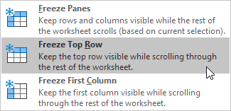
3. Scroll down to the rest of the worksheet.
Result. Excel automatically adds a dark grey horizontal line to indicate that the top row is frozen.

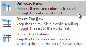
Unfreeze Panes
To unlock all rows and columns, execute the following steps.
1. On the View tab, in the Window group, click Freeze Panes.

2. Click Unfreeze Panes.
Freeze First Column
To freeze the first column, execute the following steps.
1. On the View tab, in the Window group, click Freeze Panes.

2. Click Freeze First Column.
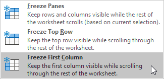
3. Scroll to the right of the worksheet.
Result. Excel automatically adds a dark grey vertical line to indicate that the first column is frozen.

Freeze Rows
To freeze rows, execute the following steps.
1. For example, select row 4.
2. On the View tab, in the Window group, click Freeze Panes.

3. Click Freeze Panes.
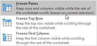
4. Scroll down to the rest of the worksheet.
Result. All rows above row 4 are frozen. Excel automatically adds a dark grey horizontal line to indicate that the first three rows are frozen.

Freeze Columns
To freeze columns, execute the following steps.
1. For example, select column E.
2. On the View tab, in the Window group, click Freeze Panes.

3. Click Freeze Panes.

4. Scroll to the right of the worksheet.
Result. All columns to the left of column E are frozen. Excel automatically adds a dark grey vertical line to indicate that the first four columns are frozen.

Freeze Cells
To freeze cells, execute the following steps.
1. For example, select cell C3.
2. On the View tab, in the Window group, click Freeze Panes.

3. Click Freeze Panes.

4. Scroll down and to the right.
Result. The orange region above row 3 and to the left of column C is frozen.

Magic Freeze Button
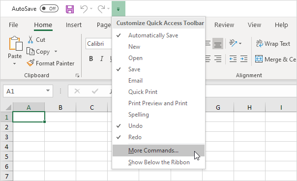
Add the magic Freeze button to the Quick Access Toolbar to freeze the top row, the first column, rows, columns or cells with a single click.
1. Click the down arrow.
2. Click More Commands.
3. Under Choose commands from, select Commands Not in the Ribbon.
4. Select Freeze Panes and click Add.
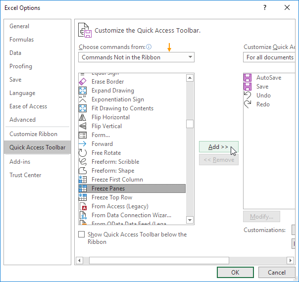
5. Click OK.
6. To freeze the top row, select row 2 and click the magic Freeze button.
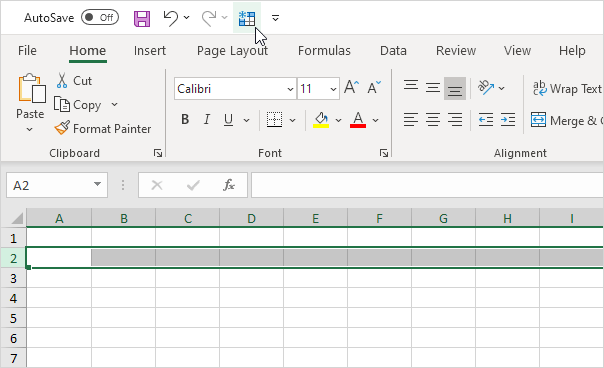
7. Scroll down to the rest of the worksheet.
Result. Excel automatically adds a dark grey horizontal line to indicate that the top row is frozen.

Note: to unlock all rows and columns, click the Freeze button again. To freeze the first 4 columns, select column E (the fifth column) and click the magic Freeze button, etc.
Tips for Using Freeze Panes Effectively
-
Always double-check your selected cell before freezing.
-
Use Freeze Panes on reports shared with teams for clarity.
-
Combine it with filters for better data control.
Conclusion
Freeze Panes in Excel is a simple yet essential tool for anyone working with large datasets. Whether you’re tracking sales, managing HR data, or preparing reports, keeping headers or key columns visible can significantly improve your workflow.
Now that you know how to use it effectively with examples, start applying it to your spreadsheets and experience the difference.