Working with multiple worksheets often leads to scattered data. Instead of analyzing each sheet one by one, you can merge the information into a single summary. In this Excel example – consolidate in Excel, you will discover how to use Excel’s built-in consolidation feature to save time and organize data effectively.
What is Data Consolidation in Excel?
Data consolidation in Excel means combining values from several ranges into a single summary table. This feature is especially useful for financial reports, sales data, or any scenario where you maintain identical tables across multiple sheets or files.
For example, if each department tracks its monthly expenses in separate worksheets, you can consolidate them into one master sheet to get the total expenses.
Why Use Consolidate in Excel?
Consolidation brings several benefits:
-
Saves time by combining data automatically.
-
Reduces errors compared to manual copy-paste.
-
Improves clarity by centralizing scattered data.
-
Supports multiple functions like Sum, Average, Count, Max, and Min.
Before you start: if your worksheets are identical, it’s probably easier to create 3D-references (if you have one workbook) or External References (if you have multiple workbooks) to consolidate your data.
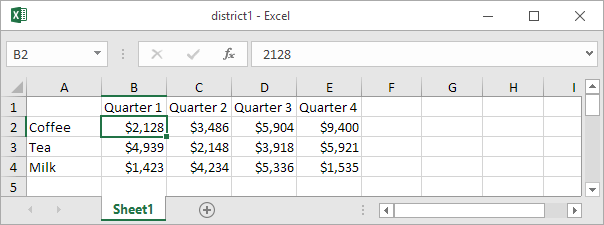
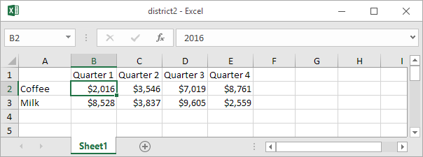
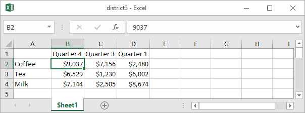
As you can see, the worksheets are not identical. However, the beauty of the Consolidate feature is that it can easily sum, count, average, etc this data by looking at the labels. This is a lot easier than creating formulas.
1. Open all three workbooks.
2. Open a blank workbook. On the Data tab, in the Data Tools group, click Consolidate.

3. Choose the Sum function to sum the data.
4. Click in the Reference box, select the range A1:E4 in the district1 workbook, and click Add.
5. Repeat step 4 for the district2 and district3 workbook.
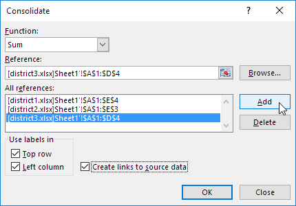
6. Check Top row, Left column and Create links to source data.
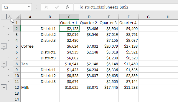
Note: if you don’t check Top row and Left column, Excel sums all cells that have the same position. For example, cell B2 (in district1.xlsx) + cell B2 (in district2.xlsx) + cell B2 (in district3.xlsx). Because our worksheets are not identical, we want Excel to sum cells that have the same labels. If you check Create links to source data, Excel creates a link to your source data (your consolidated data will be updated if your source data changes) and creates an outline.
7. Click OK.
Result.

Tips for Better Consolidation
-
Ensure consistent table layouts across all worksheets.
-
Always include headers before consolidating.
-
If ranges come from different files, open all the files before using consolidation.
-
Use links to source data if you want the consolidated sheet to update automatically when the original data changes.
Limitations of Consolidation
While powerful, consolidation has a few limits:
-
It doesn’t create pivot tables or detailed reports.
-
It works best when all worksheets have the same structure.
-
For complex data analysis, PivotTables may be more flexible.
Conclusion
This Excel example – consolidate in Excel shows how to combine data from several worksheets into one summary. By following these steps, you can quickly centralize your data, reduce errors, and analyze results with ease. Consolidation is especially handy for financial reporting, sales tracking, and any case where multiple sheets hold similar data.